Page 85 - RAC_CIAW_ a_I_n_01_2021.pdf

a set of possible solutions. At each iteration, particles
move to new positions throughout the search space,
looking for possible better solutions. The position of
each particle is updated as in (1), where x and v re-
j
j
present the position and velocity of a particle j, res-
pectively.

The velocity of each particle is computed taking
into account three main components: an inertial com-
ponent of the particle; a cognitive component that lea-
ds the particle to the best solution found by itself so far;
and a social component that leads the particle to the
best solution found by the swarm so far, considering
the knowledge of all particles. The velocity v of a par-
jd
ticle j in each dimension d is defined according to (2):

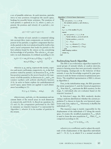
Backtracking Search Algorithm
The BSA is an evolutionary algorithm inspired by
social groups of animals which, at random intervals,
wherein: ω, φ and φ represent the inertia, cogni- return to hunting areas that were previously visited for
1 2
tive and social coefficients, respectively; m is the best food foraging. Analogously to the behavior of these
jd
position visited by particle j in dimension d; m is the animals, it uses the knowledge acquired by past gene-
gd
best position assessed by the swarm based on the expe- rations to seek for better solutions in optimization pro-
rience of all the particles, in dimension d; r and r are blems. The simplified representation of BSA is shown
2d
1d
random numbers with uniform distribution between in Algorithm 2.
[0.1]. In order to better explore the multidimensional First, in the initialization stage, the BSA generates
search space, speed limits are applied in each dimen- the initial population P and the historical population
sion d according to (3): 0
P . Note that P represents the BSA memory. In this
hist hist
stage, P individuals also are evaluated based on the
0
objective function ℱ.
wherein max and min are the maximum and mi- In Selection-I stage, the BSA randomly decides
d
d
nimum limits of the search space in each dimension (using a uniform distribution) whether the current po-
d, respectively, and δ ∈ [0, 1]. Based on equations (1), pulation P is chosen to form the new historical popu-
(2) and (3), the computation performed by the PSO lation and, thus, replace P . Afterward, it shuffles the
hist
to minimize an objective funcion ℱ is represented by individuals of P .
hist
Algorithm 1, wherein N is the number of particles in The mutation stage is mainly responsible for the
the swarm. displacement of the individuals of P along the search
space. It creates the modified population P , which
mod
is used to form the new population P new . Thus, P mod is
computed according to (4):

wherein η is a coefficient used to adjust the ampli-
tude of the displacement of the algorithm individuals
and Γ ∼ N (0, 1), in which N is a normal standard

CIAW – EFICIÊNCIA, CULTURA E TRADIÇÃO 85